Modular schedule. Function graphs with modulus

The module is one of those things that everyone seems to have heard about, but in reality no one really understands. Therefore, today there will be a big lesson dedicated to solving equations with modules.

I’ll say right away: the lesson will not be difficult. And in general, modules are a relatively simple topic. “Yes, of course, it’s not complicated! It blows my mind!” - many students will say, but all these brain breaks occur due to the fact that most people do not have knowledge in their heads, but some kind of crap. And the goal of this lesson is to turn crap into knowledge. :)

A little theory

So, let's go. Let's start with the most important thing: what is a module? Let me remind you that the modulus of a number is simply the same number, but taken without the minus sign. That is, for example, $\left| -5 \right|=5$. Or $\left| -129.5 \right|=$129.5.

Is it that simple? Yes, simple. What then is the absolute value of a positive number? It’s even simpler here: the modulus of a positive number is equal to this number itself: $\left| 5 \right|=5$; $\left| 129.5 \right|=$129.5, etc.

\[\left| -a \right|=\left| a\right|\]

Another important fact: modulus is never negative. Whatever number we take - be it positive or negative - its modulus always turns out to be positive (or, in extreme cases, zero). This is why the modulus is often called the absolute value of a number.

In addition, if we combine the definition of the modulus for a positive and negative number, we obtain a global definition of the modulus for all numbers. Namely: the modulus of a number is equal to the number itself if the number is positive (or zero), or equal to the opposite number if the number is negative. You can write this as a formula:

There is also a modulus of zero, but it is always equal to zero. In addition, zero is the only number that does not have an opposite.

Thus, if we consider the function $y=\left| x \right|$ and try to draw its graph, you will get something like this:

Modulus graph and example of solving the equation

From this picture it is immediately clear that $\left| -m \right|=\left| m \right|$, and the modulus graph never falls below the x-axis. But that’s not all: the red line marks the straight line $y=a$, which, for positive $a$, gives us two roots at once: $((x)_(1))$ and $((x)_(2)) $, but we'll talk about that later. :)

In addition to the purely algebraic definition, there is a geometric one. Let's say there are two points on the number line: $((x)_(1))$ and $((x)_(2))$. In this case, the expression $\left| ((x)_(1))-((x)_(2)) \right|$ is simply the distance between the specified points. Or, if you prefer, the length of the segment connecting these points:

Modulus is the distance between points on a number line

This definition also implies that the modulus is always non-negative. But enough definitions and theory - let's move on to real equations. :)

Basic formula

Okay, we've sorted out the definition. But that didn’t make it any easier. How to solve equations containing this very module?

Calm, just calm. Let's start with the simplest things. Consider something like this:

\[\left| x\right|=3\]

So the modulus of $x$ is 3. What could $x$ be equal to? Well, judging by the definition, we are quite happy with $x=3$. Really:

\[\left| 3\right|=3\]

Are there other numbers? Cap seems to be hinting that there is. For example, $x=-3$ is also $\left| -3 \right|=3$, i.e. the required equality is satisfied.

So maybe if we search and think, we will find more numbers? But break it off: more numbers No. Equation $\left| x \right|=3$ has only two roots: $x=3$ and $x=-3$.

Now let's complicate the task a little. Let the function $f\left(x \right)$ hang out under the modulus sign instead of the variable $x$, and put an arbitrary number $a$ in place of the triple on the right. We get the equation:

\[\left| f\left(x \right) \right|=a\]

So how can we solve this? Let me remind you: $f\left(x \right)$ is an arbitrary function, $a$ is any number. Those. Anything at all! For example:

\[\left| 2x+1 \right|=5\]

\[\left| 10x-5 \right|=-65\]

Let's pay attention to the second equation. You can immediately say about him: he has no roots. Why? Everything is correct: because it requires that the modulus be equal to a negative number, which never happens, since we already know that the modulus is always a positive number or, in extreme cases, zero.

But with the first equation everything is more fun. There are two options: either there is a positive expression under the modulus sign, and then $\left| 2x+1 \right|=2x+1$, or this expression is still negative, and then $\left| 2x+1 \right|=-\left(2x+1 \right)=-2x-1$. In the first case, our equation will be rewritten as follows:

\[\left| 2x+1 \right|=5\Rightarrow 2x+1=5\]

And suddenly it turns out that the submodular expression $2x+1$ is really positive - it is equal to the number 5. That is we can safely solve this equation - the resulting root will be a piece of the answer:

Those who are particularly distrustful can try to substitute the found root into the original equation and make sure that the modulus will actually be positive number.

Now let's look at the case of a negative submodular expression:

\[\left\( \begin(align)& \left| 2x+1 \right|=5 \\& 2x+1 \lt 0 \\\end(align) \right.\Rightarrow -2x-1=5 \Rightarrow 2x+1=-5\]

Oops! Again, everything is clear: we assumed that $2x+1 \lt 0$, and as a result we got that $2x+1=-5$ - indeed, this expression is less than zero. We solve the resulting equation, while already knowing for sure that the found root will suit us:

In total, we again received two answers: $x=2$ and $x=3$. Yes, the amount of calculations turned out to be a little larger than in the very simple equation $\left| x \right|=3$, but nothing fundamentally has changed. So maybe there is some kind of universal algorithm?

Yes, such an algorithm exists. And now we will analyze it.

Getting rid of the modulus sign

Let us be given the equation $\left| f\left(x \right) \right|=a$, and $a\ge 0$ (otherwise, as we already know, there are no roots). Then you can get rid of the modulus sign using the following rule:

\[\left| f\left(x \right) \right|=a\Rightarrow f\left(x \right)=\pm a\]

Thus, our equation with a modulus splits into two, but without a modulus. That's all the technology is! Let's try to solve a couple of equations. Let's start with this

\[\left| 5x+4 \right|=10\Rightarrow 5x+4=\pm 10\]

Let’s consider separately when there is a ten plus on the right, and separately when there is a minus. We have:

\[\begin(align)& 5x+4=10\Rightarrow 5x=6\Rightarrow x=\frac(6)(5)=1,2; \\& 5x+4=-10\Rightarrow 5x=-14\Rightarrow x=-\frac(14)(5)=-2.8. \\\end(align)\]

That's all! We got two roots: $x=1.2$ and $x=-2.8$. The entire solution took literally two lines.

Ok, no question, let's look at something a little more serious:

\[\left| 7-5x\right|=13\]

Again we open the module with plus and minus:

\[\begin(align)& 7-5x=13\Rightarrow -5x=6\Rightarrow x=-\frac(6)(5)=-1,2; \\& 7-5x=-13\Rightarrow -5x=-20\Rightarrow x=4. \\\end(align)\]

A couple of lines again - and the answer is ready! As I said, there is nothing complicated about modules. You just need to remember a few rules. Therefore, we move on and begin with truly more complex tasks.

The case of a right-hand side variable

Now consider this equation:

\[\left| 3x-2 \right|=2x\]

This equation is fundamentally different from all previous ones. How? And the fact that to the right of the equal sign is the expression $2x$ - and we cannot know in advance whether it is positive or negative.

What to do in this case? First, we must understand once and for all that if the right side of the equation turns out to be negative, then the equation will have no roots- we already know that the module cannot be equal to a negative number.

And secondly, if the right part is still positive (or equal to zero), then you can act in exactly the same way as before: simply open the module separately with a plus sign and separately with a minus sign.

Thus, we formulate a rule for arbitrary functions $f\left(x \right)$ and $g\left(x \right)$ :

\[\left| f\left(x \right) \right|=g\left(x \right)\Rightarrow \left\( \begin(align)& f\left(x \right)=\pm g\left(x \right ), \\& g\left(x \right)\ge 0. \\\end(align) \right.\]

In relation to our equation we get:

\[\left| 3x-2 \right|=2x\Rightarrow \left\( \begin(align)& 3x-2=\pm 2x, \\& 2x\ge 0. \\\end(align) \right.\]

Well, we will somehow cope with the requirement $2x\ge 0$. In the end, we can stupidly substitute the roots that we get from the first equation and check whether the inequality holds or not.

So let’s solve the equation itself:

\[\begin(align)& 3x-2=2\Rightarrow 3x=4\Rightarrow x=\frac(4)(3); \\& 3x-2=-2\Rightarrow 3x=0\Rightarrow x=0. \\\end(align)\]

Well, which of these two roots satisfies the requirement $2x\ge 0$? Yes both! Therefore, the answer will be two numbers: $x=(4)/(3)\;$ and $x=0$. That's the solution. :)

I suspect that some of the students are already starting to get bored? Well, let's look at an even more complex equation:

\[\left| ((x)^(3))-3((x)^(2))+x \right|=x-((x)^(3))\]

Although it looks evil, in fact it is still the same equation of the form “modulus equals function”:

\[\left| f\left(x \right) \right|=g\left(x \right)\]

And it is solved in exactly the same way:

\[\left| ((x)^(3))-3((x)^(2))+x \right|=x-((x)^(3))\Rightarrow \left\( \begin(align)& ( (x)^(3))-3((x)^(2))+x=\pm \left(x-((x)^(3)) \right), \\& x-((x )^(3))\ge 0. \\\end(align) \right.\]

We will deal with inequality later - it is somehow too evil (in fact, it is simple, but we will not solve it). For now, it’s better to deal with the resulting equations. Let's consider the first case - this is when the module is expanded with a plus sign:

\[((x)^(3))-3((x)^(2))+x=x-((x)^(3))\]

Well, it’s a no brainer that you need to collect everything from the left, bring similar ones and see what happens. And this is what happens:

\[\begin(align)& ((x)^(3))-3((x)^(2))+x=x-((x)^(3)); \\& 2((x)^(3))-3((x)^(2))=0; \\\end(align)\]

We take it out common multiplier$((x)^(2))$ out of brackets and we get a very simple equation:

\[((x)^(2))\left(2x-3 \right)=0\Rightarrow \left[ \begin(align)& ((x)^(2))=0 \\& 2x-3 =0 \\\end(align) \right.\]

\[((x)_(1))=0;\quad ((x)_(2))=\frac(3)(2)=1.5.\]

Here we took advantage of an important property of the product, for the sake of which we factored the original polynomial: the product is equal to zero when at least one of the factors is equal to zero.

Now let’s deal with the second equation in exactly the same way, which is obtained by expanding the module with a minus sign:

\[\begin(align)& ((x)^(3))-3((x)^(2))+x=-\left(x-((x)^(3)) \right); \\& ((x)^(3))-3((x)^(2))+x=-x+((x)^(3)); \\& -3((x)^(2))+2x=0; \\& x\left(-3x+2 \right)=0. \\\end(align)\]

Again the same thing: the product is equal to zero when at least one of the factors is equal to zero. We have:

\[\left[ \begin(align)& x=0 \\& -3x+2=0 \\\end(align) \right.\]

Well, we got three roots: $x=0$, $x=1.5$ and $x=(2)/(3)\;$. Well, which of this set will go into the final answer? To do this, remember that we have an additional constraint in the form of inequality:

How to take this requirement into account? Let’s just substitute the found roots and check whether the inequality holds for these $x$ or not. We have:

\[\begin(align)& x=0\Rightarrow x-((x)^(3))=0-0=0\ge 0; \\& x=1.5\Rightarrow x-((x)^(3))=1.5-((1.5)^(3)) \lt 0; \\& x=\frac(2)(3)\Rightarrow x-((x)^(3))=\frac(2)(3)-\frac(8)(27)=\frac(10) (27)\ge 0; \\\end(align)\]

Thus, the root $x=1.5$ does not suit us. And in response there will be only two roots:

\[((x)_(1))=0;\quad ((x)_(2))=\frac(2)(3).\]

As you can see, even in this case there was nothing complicated - equations with modules are always solved using an algorithm. You just need to have a good understanding of polynomials and inequalities. Therefore, we move on to more complex tasks - there will already be not one, but two modules.

Equations with two modules

So far we have studied only the most simple equations— there was one module and something else. We sent this “something else” to another part of the inequality, away from the module, so that in the end everything would be reduced to an equation of the form $\left| f\left(x \right) \right|=g\left(x \right)$ or even simpler $\left| f\left(x \right) \right|=a$.

But kindergarten ended - it's time to consider something more serious. Let's start with equations like this:

\[\left| f\left(x \right) \right|=\left| g\left(x \right) \right|\]

This is an equation of the form “modulus equal to modulus" The fundamentally important point is the absence of other terms and factors: only one module on the left, one more module on the right - and nothing more.

Someone will now think that such equations are more difficult to solve than what we have studied so far. But no: these equations are even easier to solve. Here's the formula:

\[\left| f\left(x \right) \right|=\left| g\left(x \right) \right|\Rightarrow f\left(x \right)=\pm g\left(x \right)\]

All! We simply equate submodular expressions by putting a plus or minus sign in front of one of them. And then we solve the resulting two equations - and the roots are ready! No additional restrictions, no inequalities, etc. Everything is very simple.

Let's try to solve this problem:

\[\left| 2x+3 \right|=\left| 2x-7 \right|\]

Elementary Watson! Expanding the modules:

\[\left| 2x+3 \right|=\left| 2x-7 \right|\Rightarrow 2x+3=\pm \left(2x-7 \right)\]

Let's consider each case separately:

\[\begin(align)& 2x+3=2x-7\Rightarrow 3=-7\Rightarrow \emptyset ; \\& 2x+3=-\left(2x-7 \right)\Rightarrow 2x+3=-2x+7. \\\end(align)\]

The first equation has no roots. Because when is $3=-7$? At what values of $x$? “What the hell is $x$? Are you stoned? There’s no $x$ there at all,” you say. And you'll be right. We have obtained an equality that does not depend on the variable $x$, and at the same time the equality itself is incorrect. That's why there are no roots. :)

With the second equation, everything is a little more interesting, but also very, very simple:

As you can see, everything was solved literally in a couple of lines - we didn’t expect anything else from a linear equation. :)

As a result, the final answer is: $x=1$.

So how? Difficult? Of course not. Let's try something else:

\[\left| x-1 \right|=\left| ((x)^(2))-3x+2 \right|\]

Again we have an equation of the form $\left| f\left(x \right) \right|=\left| g\left(x \right) \right|$. Therefore, we immediately rewrite it, revealing the modulus sign:

\[((x)^(2))-3x+2=\pm \left(x-1 \right)\]

Perhaps someone will now ask: “Hey, what nonsense? Why does “plus-minus” appear on the right-hand expression and not on the left?” Calm down, I’ll explain everything now. Indeed, in a good way we should have rewritten our equation as follows:

Then you need to open the brackets, move all the terms to one side of the equal sign (since the equation, obviously, will be square in both cases), and then find the roots. But you must admit: when “plus-minus” appears before three terms (especially when one of these terms is a quadratic expression), it somehow looks more complicated than the situation when “plus-minus” appears before only two terms.

But nothing prevents us from rewriting the original equation as follows:

What happened? Nothing special: they just changed the left one and right side in some places. A little thing that will ultimately make our life a little easier. :)

In general, we solve this equation, considering options with a plus and a minus:

\[\begin(align)& ((x)^(2))-3x+2=x-1\Rightarrow ((x)^(2))-4x+3=0; \\& ((x)^(2))-3x+2=-\left(x-1 \right)\Rightarrow ((x)^(2))-2x+1=0. \\\end(align)\]

The first equation has roots $x=3$ and $x=1$. The second is generally an exact square:

\[((x)^(2))-2x+1=((\left(x-1 \right))^(2))\]

Therefore, it has only one root: $x=1$. But we have already obtained this root earlier. Thus, only two numbers will go into the final answer:

\[((x)_(1))=3;\quad ((x)_(2))=1.\]

Mission Complete! You can take a pie from the shelf and eat it. There are 2 of them, yours is the middle one. :)

Important Note. The presence of identical roots for different variants of expansion of the module means that the original polynomials are factorized, and among these factors there will definitely be a common one. Really:

\[\begin(align)& \left| x-1 \right|=\left| ((x)^(2))-3x+2 \right|; \\& \left| x-1 \right|=\left| \left(x-1 \right)\left(x-2 \right) \right|. \\\end(align)\]

One of the module properties: $\left| a\cdot b \right|=\left| a \right|\cdot \left| b \right|$ (i.e. the modulus of the product is equal to the product of the moduli), so the original equation can be rewritten as follows:

\[\left| x-1 \right|=\left| x-1 \right|\cdot \left| x-2 \right|\]

As you can see, we really have a common factor. Now, if you collect all the modules on one side, you can take this factor out of the bracket:

\[\begin(align)& \left| x-1 \right|=\left| x-1 \right|\cdot \left| x-2 \right|; \\& \left| x-1 \right|-\left| x-1 \right|\cdot \left| x-2 \right|=0; \\& \left| x-1 \right|\cdot \left(1-\left| x-2 \right| \right)=0. \\\end(align)\]

Well, now remember that the product is equal to zero when at least one of the factors is equal to zero:

\[\left[ \begin(align)& \left| x-1 \right|=0, \\& \left| x-2 \right|=1. \\\end(align) \right.\]

Thus, the original equation with two modules has been reduced to the two simplest equations that we talked about at the very beginning of the lesson. Such equations can be solved literally in a couple of lines. :)

This remark may seem unnecessarily complex and inapplicable in practice. However, in reality, you may encounter much more complex problems than those we are looking at today. In them, modules can be combined with polynomials, arithmetic roots, logarithms, etc. And in such situations, the ability to lower the overall degree of the equation by taking something out of brackets can be very, very useful. :)

Now I would like to look at another equation, which at first glance may seem crazy. Many students get stuck on it, even those who think they have a good understanding of the modules.

However, this equation is even easier to solve than what we looked at earlier. And if you understand why, you will get another trick for quick solution equations with modules.

So the equation is:

\[\left| x-((x)^(3)) \right|+\left| ((x)^(2))+x-2 \right|=0\]

No, this is not a typo: it is a plus between the modules. And we need to find at what $x$ the sum of two modules is equal to zero. :)

What's the problem anyway? But the problem is that each module is a positive number, or, in extreme cases, zero. What happens if you add two positive numbers? Obviously a positive number again:

\[\begin(align)& 5+7=12 \gt 0; \\& 0.004+0.0001=0.0041 \gt 0; \\& 5+0=5 \gt 0. \\\end(align)\]

The last line might give you an idea: the only time the sum of the modules is zero is if each module is zero:

And when is the module equal to zero? Only in one case - when the submodular expression is equal to zero:

\[((x)^(2))+x-2=0\Rightarrow \left(x+2 \right)\left(x-1 \right)=0\Rightarrow \left[ \begin(align)& x=-2 \\& x=1 \\\end(align) \right.\]

Thus, we have three points at which the first module is reset to zero: 0, 1 and −1; as well as two points at which the second module is reset to zero: −2 and 1. However, we need both modules to be reset to zero at the same time, so among the found numbers we need to choose those that are included in both sets. Obviously, there is only one such number: $x=1$ - this will be the final answer.

Cleavage method

Well, we've already covered a bunch of problems and learned a lot of techniques. Do you think that's all? But no! Now we will look at the final technique - and at the same time the most important. We will talk about splitting equations with modulus. What will we even talk about? Let's go back a little and look at some simple equation. For example this:

\[\left| 3x-5 \right|=5-3x\]

In principle, we already know how to solve such an equation, because it is a standard construction of the form $\left| f\left(x \right) \right|=g\left(x \right)$. But let's try to look at this equation from a slightly different angle. More precisely, consider the expression under the modulus sign. Let me remind you that the modulus of any number can be equal to the number itself, or it can be opposite to this number:

\[\left| a \right|=\left\( \begin(align)& a,\quad a\ge 0, \\& -a,\quad a \lt 0. \\\end(align) \right.\]

Actually, this ambiguity is the whole problem: since the number under the modulus changes (it depends on the variable), it is not clear to us whether it is positive or negative.

But what if you initially require that this number be positive? For example, let's require that $3x-5 \gt 0$ - in this case we are guaranteed to get a positive number under the modulus sign, and we can completely get rid of this very modulus:

Thus, our equation will turn into a linear one, which can be easily solved:

True, all these thoughts make sense only under the condition $3x-5 \gt 0$ - we ourselves introduced this requirement in order to unambiguously reveal the module. Therefore, let's substitute the found $x=\frac(5)(3)$ into this condition and check:

It turns out that for the specified value of $x$ our requirement is not met, because the expression turned out to be equal to zero, and we need it to be strictly greater than zero. Sad. :(

But it's okay! After all, there is another option $3x-5 \lt 0$. Moreover: there is also the case $3x-5=0$ - this also needs to be considered, otherwise the solution will be incomplete. So, consider the case $3x-5 \lt 0$:

Obviously, the module will open with a minus sign. But then a strange situation arises: both on the left and on the right in the original equation the same expression will stick out:

I wonder at what $x$ the expression $5-3x$ will be equal to the expression $5-3x$? Even Captain Obviousness would choke on his saliva from such equations, but we know: this equation is an identity, i.e. it is true for any value of the variable!

This means that any $x$ will suit us. However, we have a limitation:

In other words, the answer will not be a single number, but a whole interval:

Finally, there is one more case left to consider: $3x-5=0$. Everything is simple here: under the modulus there will be zero, and the modulus of zero is also equal to zero (this follows directly from the definition):

But then the original equation $\left| 3x-5 \right|=5-3x$ will be rewritten as follows:

We already obtained this root above when we considered the case of $3x-5 \gt 0$. Moreover, this root is a solution to the equation $3x-5=0$ - this is the limitation that we ourselves introduced to reset the module. :)

Thus, in addition to the interval, we will also be satisfied with the number lying at the very end of this interval:

Combining roots in modulo equations

Total final answer: $x\in \left(-\infty ;\frac(5)(3) \right]$ It’s not very common to see such crap in the answer to a fairly simple (essentially linear) equation with modulus , really? Well, get used to it: the difficulty of the module is that the answers in such equations can turn out to be completely unpredictable.

Something else is much more important: we have just analyzed a universal algorithm for solving an equation with a modulus! And this algorithm consists of the following steps:

Equate each modulus in the equation to zero. We get several equations;
Solve all these equations and mark the roots on the number line. As a result, the straight line will be divided into several intervals, at each of which all modules are uniquely revealed;
Solve the original equation for each interval and combine your answers.

That's all! There is only one question left: what to do with the roots obtained in step 1? Let's say we have two roots: $x=1$ and $x=5$. They will split the number line into 3 pieces:

Splitting the number line into intervals using points

So what are the intervals? It is clear that there are three of them:

The leftmost one: $x \lt 1$ — the unit itself is not included in the interval;
Central: $1\le x \lt 5$ - here one is included in the interval, but five is not included;
Rightmost: $x\ge 5$ - five is only included here!

I think you already understand the pattern. Each interval includes the left end and does not include the right.

At first glance, such an entry may seem inconvenient, illogical and generally some kind of crazy. But believe me: after a little practice, you will find that this approach is the most reliable and does not interfere with unambiguously opening the modules. It’s better to use such a scheme than to think every time: give the left/right end to the current interval or “throw” it into the next one.

This concludes the lesson. Download problems to solve on your own, practice, compare with the answers - and see you in the next lesson, which will be devoted to inequalities with moduli. :)

Function of the form y=|x|.
The graph of a function on an interval is with the graph of the function y=-x.

Let's first consider the simplest case - the function y=|x|. By definition of a module, we have:

Thus, for x≥0 the function y=|x| coincides with the function y=x, and for x Using this explanation, it is easy to plot the function y=|x| (Fig. 1).

It is easy to see that this graph is a combination of that part of the graph of the function y = x that lies not below the OX axis and the line obtained by mirror reflection relative to the OX axis, that part that lies below the OX axis.
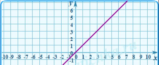
This method is also suitable for plotting the function y=|kx+b|.
If the graph of the function y=kx+b is shown in Fig. 2, then the graph of the function y=|kx+b| is the line shown in Fig. 3.

Example 1. Graph the function y=||1-x 2 |-3|.
Let's build a graph of the function y=1-x 2 and apply the “modulus” operation to it (the part of the graph located below the OX axis is symmetrically reflected relative to the OX axis).

Let's shift the graph down by 3.

Let's apply the "modulus" operation and get the final graph of the function y=||1-x 2 |-3|

Example 2. Construct a graph of the function y=||x 2 -2x|-3|.
As a result of the transformation, we obtain y=|x 2 -2x|=|(x-1) 2 -1|. Let's build a graph of the function y=(x-1) 2 -1: build a parabola y=x 2 and shift to the right by 1 and down by 1.

Let’s apply the “modulus” operation to it (the part of the graph located below the OX axis is symmetrically reflected relative to the OX axis).

Let's shift the graph down by 3 and apply the “modulus” operation, resulting in the final graph.

Example 3. Construct a graph of the function.
To expand the module, we need to consider two cases:
1)x>0, then the module will open with a “+” sign =
2)x =

Let's build a graph for the first case.

Let's discard the part of the graph where x

Let's build a graph for the second case and similarly discard the part where x>0, as a result we get.

Let's connect the two graphs and get the final one.

Example 4. Construct a graph of the function.
Let's first construct a graph of the function. To do this, it is convenient to select the whole part, we get . Building on the table of values, we get a graph.

Let's apply the modulus operation (the part of the graph located below the OX axis is symmetrically reflected relative to the OX axis). We get the final schedule

Example 5. Graph the function y=|-x 2 +6x-8|. First, let's simplify the function to y=1-(x-3) 2 and build its graph

Now we will apply the “modulus” operation and display the part of the graph below the OX axis, relative to the OX axis

Example 6. Draw a graph of the function y=-x 2 +6|x|-8. Let’s also simplify the function to y=1-(x-3) 2 and plot it

Now we will apply the “modulus” operation and reflect the part of the graph to the right of the oY axis, to the left side

Example 7. Graph the function . Let's plot the function

Let's plot the function

Let's carry out a parallel translation of 3 unit segments to the right and 2 up. The graph will look like:

Let's apply the "modulus" operation and reflect the part of the graph to the right of the straight line x=3 into the left half-plane.

Transcript

1 Regional scientific-practical conference educational and research works of students in grades 6-11 “Applied and fundamental issues of mathematics” Methodological aspects of studying mathematics Construction of graphs of functions containing the module Gabova Angela Yuryevna, 10th grade, MOBU “Gymnasium 3” Kudymkar, Pikuleva Nadezhda Ivanovna, mathematics teacher MOBU “ Gymnasium 3" Kudymkar Perm, 2016

2 Contents: Introduction...3 p. I. Main part...6 p. 1.1 Historical reference.. 6 page 2.Basic definitions and properties of functions page 2.1 Quadratic function..7 page 2.2 Linear function...8 page 2.3 Fractional-rational function 8 page 3. Algorithms for constructing graphs with a modulus 9 pages 3.1 Definition of the module.. 9 pages 3.2 Algorithm for constructing a graph linear function with module...9 p. 3.3 Constructing graphs of functions containing “nested modules” in the formula.10 p. 3.4 Algorithm for constructing graphs of functions of the form y = a 1 x x 1 + a 2 x x a n x x n + ax + b...13 p. 3.5 Algorithm for constructing a graph of a quadratic function with modulus. 14 p. 3.6 Algorithm for constructing a graph of a fractional rational function with modulus. 15pp. 4. Changes in the graph of a quadratic function depending on the location of the sign of the absolute value..17p. II. Conclusion...26 pp. III. List of references and sources...27 pp. IV. Appendix....28pp. 2

3 Introduction Graphing functions is one of them the most interesting topics in school mathematics. The greatest mathematician of our time, Israel Moiseevich Gelfand, wrote: “The process of constructing graphs is a way of transforming formulas and descriptions into geometric images. This graphing is a means of seeing formulas and functions and seeing how those functions change. For example, if it is written y =x 2, then you immediately see a parabola; if y = x 2-4, you see a parabola lowered by four units; if y = -(x 2 4), then you see the previous parabola turned down. This ability to immediately see a formula and its geometric interpretation is important not only for studying mathematics, but also for other subjects. It’s a skill that stays with you for life, like riding a bike, typing, or driving a car.” The basics of solving equations with modules were obtained in the 6th-7th grades. I chose this particular topic because I believe that it requires deeper and more thorough research. I want to gain more knowledge about the modulus of numbers, in various ways constructing graphs containing the sign of the absolute value. When the modulus sign is included in “standard” equations of lines, parabolas, and hyperbolas, their graphs become unusual and even beautiful. To learn how to build such graphs, you need to master the techniques of constructing basic figures, as well as firmly know and understand the definition of the modulus of a number. In the school mathematics course, graphs with the module are not discussed in depth enough, which is why I wanted to expand my knowledge on this topic and conduct my own research. Without knowing the definition of a modulus, it is impossible to construct even the simplest graph containing an absolute value. Characteristic feature graphs of functions containing expressions with a modulus sign, 3

4 is the presence of kinks at those points at which the expression under the modulus sign changes sign. Purpose of the work: to consider the construction of a graph of linear, quadratic and fractionally rational functions containing a variable under the modulus sign. Objectives: 1) Study the literature on the properties of the absolute value of linear, quadratic and fractional-rational functions. 2) Investigate changes in function graphs depending on the location of the sign of the absolute value. 3) Learn to graph equations. Object of study: graphs of linear, quadratic and fractionally rational functions. Subject of research: changes in the graph of linear, quadratic and fractionally rational functions depending on the location of the sign of the absolute value. The practical significance of my work lies in: 1) using the acquired knowledge on this topic, as well as deepening it and applying it to other functions and equations; 2) in the use of skills research work in the future educational activities. Relevance: Graphing tasks are traditionally one of the most difficult topics in mathematics. Our graduates are faced with the problem of successfully passing the State Exam and the Unified State Exam. Research problem: constructing graphs of functions containing the modulus sign from the second part of the GIA. Research hypothesis: the use of a methodology for solving tasks in the second part of the GIA, developed on the basis of general methods for constructing graphs of functions containing a modulus sign, will allow students to solve these tasks 4

5 on a conscious basis, choose the most rational method of solution, apply different methods of solution and pass the State Exam more successfully. Research methods used in the work: 1. Analysis of mathematical literature and Internet resources on this topic. 2. Reproductive reproduction of the studied material. 3. Cognitive and search activities. 4.Analysis and comparison of data in search of solutions to problems. 5. Statement of hypotheses and their verification. 6. Comparison and generalization of mathematical facts. 7. Analysis of the results obtained. When writing this work, the following sources were used: Internet resources, OGE tests, mathematical literature. 5

6 I. Main part 1.1 Historical background. In the first half of the 17th century, the idea of function as a dependence of one variable size from another. Thus, the French mathematicians Pierre Fermat () and Rene Descartes () imagined a function as the dependence of the ordinate of a point on a curve on its abscissa. And the English scientist Isaac Newton () understood a function as the coordinate of a moving point changing depending on time. The term “function” (from the Latin function execution, accomplishment) was first introduced by the German mathematician Gottfried Leibniz(). He associated a function with a geometric image (the graph of a function). Subsequently, the Swiss mathematician Johann Bernoulli() and a member of the St. Petersburg Academy of Sciences, the famous 18th-century mathematician Leonard Euler(), considered the function as an analytical expression. Euler also has a general understanding of a function as the dependence of one variable on another. The word “module” comes from the Latin word “modulus”, which means “measure”. This ambiguous word(homonym), which has many meanings and is used not only in mathematics, but also in architecture, physics, technology, programming and other exact sciences. In architecture, this is the initial unit of measurement established for a given architectural structure and used to express multiple ratios of its constituent elements. In technology, this is a term used in various fields of technology, which does not have a universal meaning and serves to designate various coefficients and quantities, for example, engagement modulus, elastic modulus, etc. 6

7 Bulk modulus (in physics) is the ratio of normal stress in a material to relative elongation. 2. Basic definitions and properties of functions Function is one of the most important mathematical concepts. A function is a dependence of the variable y on the variable x such that each value of the variable x corresponds to a single value of the variable y. Methods for specifying a function: 1) analytical method (the function is specified using mathematical formula); 2) tabular method (the function is specified using a table); 3) descriptive method (the function is specified verbal description); 4) graphical method (the function is specified using a graph). The graph of a function is the set of all points coordinate plane, the abscissas of which are equal to the value of the argument, and the ordinates are equal to the corresponding values of the function. 2.1 Quadratic function A function defined by the formula y = ax 2 + in + c, where x and y are variables, and the parameters a, b and c are any real numbers, and a = 0, is called quadratic. The graph of the function y=ax 2 +in+c is a parabola; the axis of symmetry of the parabola y=ax 2 +in+c is a straight line, for a>0 the “branches” of the parabola are directed upward, for a<0 вниз. Чтобы построить график квадратичной функции, нужно: 1) найти координаты вершины параболы и отметить её в координатной плоскости; 2) построить ещё несколько точек, принадлежащих параболе; 3) соединить отмеченные точки плавной линией.,. 2.2Линейная функция функция вида 7

8 (for functions of one variable). The main property of linear functions: the increment of the function is proportional to the increment of the argument. That is, the function is a generalization of direct proportionality. The graph of a linear function is a straight line, which is where its name comes from. This concerns a real function of one real variable. 1) When, the straight line forms an acute angle with the positive direction of the abscissa axis. 2) When, the straight line forms an obtuse angle with the positive direction of the x-axis. 3) is the ordinate indicator of the point of intersection of the line with the ordinate axis. 4) When, the straight line passes through the origin. , 2.3 A fractional-rational function is a fraction whose numerator and denominator are polynomials. It has the form where, polynomials in any number of variables. A special case is rational functions of one variable:, where and are polynomials. 1) Any expression that can be obtained from variables using four arithmetic operations is a rational function. 8

9 2) The set of rational functions is closed under arithmetic operations and the composition operation. 3) Any rational function can be represented as a sum of simple fractions - this is used in analytical integration.. , 3. Algorithms for constructing graphs with modulus 3.1 Definition of modulus The modulus of a real number a is the number a itself, if it is non-negative, and the number opposite a, if a is negative. a = 3.2 Algorithm for constructing a graph of a linear function with modulus To construct graphs of functions y = x you need to know that for positive x we have x = x. This means that for positive values of the argument, the graph y= x coincides with the graph y=x, that is, this part of the graph is a ray emerging from the origin at an angle of 45 degrees to the abscissa axis. At x< 0 имеем x = -x; значит, для отрицательных x график y= x совпадает с биссектрисой второго координатного угла. Впрочем, вторую половину графика (для отрицательных X) легко получить из первой, если заметить, что функция y= x чётная, так как -a = a. Значит, график функции y= x симметричен относительно оси Oy, и вторую половину графика можно приобрести, отразив относительно оси ординат часть, начерченную для положительных x. Получается график:y= x 9

10 To construct, we take points (-2; 2) (-1; 1) (0; 0) (1; 1) (2; 2). Now let’s build a graph y= x-1. If A is a point on the graph y= x with coordinates (a; a), then the point on the graph y= x-1 with the same value of the Y ordinate will be point A1(a+1; a). This point of the second graph can be obtained from point A(a; a) of the first graph by shifting parallel to the Ox axis to the right. This means that the entire graph of the function y= x-1 is obtained from the graph of the function y= x by shifting parallel to the Ox axis to the right by 1. Let’s construct the graphs: y= x-1 To construct, take the points (-2; 3) (-1; 2) (0; 1) (1; 0) (2; 1). 3.3 Constructing graphs of functions containing “nested modules” in the formula Let’s consider the construction algorithm using a specific example Construct a graph of a function: 10

11 y=i-2-ix+5ii 1. Build a graph of the function. 2. We display the graph of the lower half-plane upward symmetrically relative to the OX axis and obtain the graph of the function. eleven

12 3. We display the graph of the function downwards symmetrically relative to the OX axis and obtain the graph of the function. 4. We display the graph of the function downwards symmetrically relative to the OX axis and obtain a graph of the function 5. We display the graph of the function relative to the OX axis and obtain a graph. 12

13 6. As a result, the graph of the function looks like this 3.4. Algorithm for constructing graphs of functions of the form y = a 1 x x 1 + a 2 x x a n x x n + ax + b. In the previous example, it was quite easy to reveal the modulus signs. If there are more sums of modules, then it is problematic to consider all possible combinations of signs of submodular expressions. How, in this case, to construct a graph of the function? Note that the graph is a broken line, with vertices at points having abscissas -1 and 2. At x = -1 and x = 2, the submodular expressions are equal to zero. In a practical way, we have come closer to the rule for constructing such graphs: The graph of a function of the form y = a 1 x x 1 + a 2 x x a n x x n + ax + b is a broken line with infinite extreme links. To construct such a broken line, it is enough to know all its vertices (the abscissas of the vertices are the zeros of the submodular expressions) and one control point on the left and right infinite links. 13

14 Problem. Graph the function y = x + x 1 + x + 1 and find its smallest value. Solution: 1. Zeros of submodular expressions: 0; -1; Vertices of the polyline (0; 2); (-13); (1; 3). (we substitute the zeros of the submodular expressions into the equation) 3 Check point on the right (2; 6), on the left (-2; 6). We build a graph (Fig. 7), the smallest value of the function is Algorithm for constructing a graph of a quadratic function with the module Drawing up algorithms for converting function graphs. 1. Plotting a graph of the function y= f(x). By definition of a module, this function is divided into a set of two functions. Consequently, the graph of the function y= f(x) consists of two graphs: y= f(x) in the right half-plane, y= f(-x) in the left half-plane. Based on this, a rule (algorithm) can be formulated. The graph of the function y= f(x) is obtained from the graph of the function y= f(x) as follows: at x 0 the graph is preserved, and at x< 0полученная часть графика отображается симметрично относительно оси ОУ. 2.Построение графика функции y= f(x). а). Строим график функции y= f(x). б). Часть графика y= f(x), лежащая над осью ОХ, сохраняется, часть его, лежащая под осью ОХ, отображается симметрично относительно оси ОХ. 14

15 3. To build a graph of the function y= f(x), you must first build a graph of the function y= f(x) for x> 0, then for x< 0 построить изображение, симметричное ему относительно оси ОУ, а затем на интервалах, где f(x) <0,построить изображение, симметричное графику y= f(x) относительно оси ОХ. 4.Для построения графиков вида y = f(x)достаточно построить график функции y= f(x) для тех х из области определения, при которых f(х) 0, и отобразить полученную часть графика симметрично относительно оси абсцисс. Пример Построим график функции у = х 2 6х +5. Сначала построим параболу у= х 2 6х +5. Чтобы получить из неё график функции у = х 2-6х + 5, нужно каждую точку параболы с отрицательной ординатой заменить точкой с той же абсциссой, но с противоположной (положительной) ординатой. Иными словами, часть параболы, расположенную ниже оси Ох, нужно заменить линией, ей симметричной относительно оси Ох (Рис.1). Рис Алгоритм построения графика дробно рациональной функции с модулем 1. Начнем с построения графика В основе его лежит график функции и все мы знаем, как он выглядит: Теперь построим график 15

16 To get this graph, you just need to shift the previously obtained graph three units to the right. Note that if the denominator of the fraction contained the expression x + 3, then we would shift the graph to the left: Now we need to multiply all ordinates by two to get the graph of the function. Finally, we shift the graph up by two units: The last thing we have to do is , this is to plot a graph of a given function if it is enclosed under the modulus sign. To do this, we reflect symmetrically upward the entire part of the graph whose ordinates are negative (that part that lies below the x-axis): Fig. 4 16

17 4.Changes in the graph of a quadratic function depending on the location of the sign of the absolute value. Construct a graph of the function y = x 2 - x -3 1) Since x = x at x 0, the required graph coincides with the parabola y = 0.25 x 2 - x - 3. If x<0, то поскольку х 2 = х 2, х =-х и требуемый график совпадает с параболой у=0,25 х 2 + х) Если рассмотрим график у=0,25 х 2 - х - 3 при х 0 и отобразить его относительно оси ОУ мы получим тот же самый график. (0; - 3) координаты точки пересечения графика функции с осью ОУ. у =0, х 2 -х -3 = 0 х 2-4х -12 = 0 Имеем, х 1 = - 2; х 2 = 6. (-2; 0) и (6; 0) - координаты точки пересечения графика функции с осью ОХ. Если х<0, ордината точки требуемого графика такая же, как и у точки параболы, но с положительной абсциссой, равной х. Такие точки симметричны относительно оси ОУ(например, вершины (2; -4) и -(2; -4). Значит, часть требуемого графика, соответствующая значениям х<0, симметрична относительно оси ОУ его же части, соответствующей значениям х>0. b) Therefore, I complete the construction for x<0 часть графика, симметричную построенной относительно оси ОУ. 17

18 Fig. 4 The graph of the function y = f (x) coincides with the graph of the function y = f (x) on the set of non-negative values of the argument and is symmetrical to it with respect to the axis of the OU on the set of negative values of the argument. Proof: If x 0, then f (x) = f (x), i.e. on the set of non-negative values of the argument, the graphs of the functions y = f (x) and y = f (x) coincide. Since y = f (x) is an even function, its graph is symmetrical with respect to the op-amp. Thus, the graph of the function y = f (x) can be obtained from the graph of the function y = f (x) as follows: 1. construct a graph of the function y = f (x) for x>0; 2. For x<0, симметрично отразить построенную часть относительно оси ОУ. Вывод: Для построения графика функции у = f (х) 1. построить график функции у = f(х) для х>0; 2. For x<0, симметрично отразить построенную часть относительно оси ОУ. Построить график функции у = х 2-2х Освободимся от знака модуля по определению Если х 2-2х 0, т.е. если х 0 и х 2, то х 2-2х = х 2-2х Если х 2-2х<0, т.е. если 0<х< 2, то х 2-2х =- х 2 + 2х Видим, что на множестве х 0 и х 2 графики функции у = х 2-2х и у = х 2-2х совпадают, а на множестве (0;2) графики функции у = -х 2 + 2х и у = х 2-2х совпадают. Построим их. График функции у = f (х) состоит из части графика функции у = f(х) при у?0 и симметрично отражённой части у = f(х) при у <0 относительно оси ОХ. Построить график функции у = х 2 - х -6 1) Если х 2 - х -6 0, т.е. если х -2 и х 3, то х 2 - х -6 = х 2 - х

19 If x 2 - x -6<0, т.е. если -2<х< 3, то х 2 - х -6 = -х 2 + х +6. Построим их. 2) Построим у = х 2 - х -6. Нижнюю часть графика симметрично отбражаем относительно ОХ. Сравнивая 1) и 2), видим что графики одинаковые. Работа на тетрадях. Докажем, что график функции у = f (х) совпадает с графиком функции у = f (х) для f(х) >0 and symmetrically reflected part y = f(x) at y<0 относительно оси ОХ. Действительно, по определению абсолютной величины, можно данную функцию рассмотреть как совокупность двух линий: у = f(х), если f(х) 0; у = - f(х), если f(х) <0 Для любой функции у = f(х), если f(х) >0, then f (x) = f (x), which means in this part the graph of the function y = f (x) coincides with the graph of the function itself y = f (x). If f(x)<0, то f (х) = - f(х),т.е. точка (х; - f(х)) симметрична точке (х; f (х)) относительно оси ОХ. Поэтому для получения требуемого графика отражаем симметрично относительно оси ОХ "отрицательную" часть графика у = f(х). Вывод: действительно для построения графика функции у = f(х) достаточно: 1.Построить график функции у = f(х) ; 2. На участках, где график расположен в нижней полуплоскости, т.е., где f(х) <0, симметрично отражаем относительно оси абсцисс. (Рис.5) 19

20 Fig.5 Conclusion: To build a graph of the function y= f(x) 1. Build a graph of the function y=f(x) ; 2. In areas where the graph is located in the lower half-plane, i.e., where f(x)<0, строим кривые, симметричные построенным графикам относительно оси абсцисс. (Рис.6, 7.) 20

21 Research work on constructing graphs of the function y = f (x) Using the definition of absolute value and previously discussed examples, we will construct graphs of the function: y = 2 x - 3 y = x 2-5 x y = x 2-2 and draw conclusions. In order to build a graph of the function y = f (x) you need to: 1. Build a graph of the function y = f (x) for x>0. 2. Construct the second part of the graph, i.e. reflect the constructed graph symmetrically relative to the op-amp, because This function is even. 3. Convert sections of the resulting graph located in the lower half-plane to the upper half-plane symmetrically to the OX axis. Construct a graph of the function y = 2 x - 3 (1st method for determining the modulus) 1. Construct y = 2 x - 3, for 2 x - 3 > 0, x >1.5 i.e. X< -1,5 и х>1.5 a) y = 2x - 3, for x>0 b) for x<0, симметрично отражаем построенную часть относительно оси ОУ. 2. Строим у = -2 х + 3, для 2 х - 3 < 0. т.е. -1,5<х<1,5 а) у = -2х + 3, для х>0 b) for x<0, симметрично отражаем построенную часть относительно оси ОУ. У = 2 х - 3 1) Строим у = 2х-3, для х>0. 2) We construct a straight line, symmetrical to the one constructed relative to the axis of the op-amp. 3) I display sections of the graph located in the lower half-plane symmetrically relative to the OX axis. Comparing both graphs, we see that they are the same. 21

22 Examples of problems Example 1. Consider the graph of the function y = x 2 6x +5. Since x is squared, regardless of the sign of the number x, after squaring it will be positive. It follows that the graph of the function y = x 2-6x +5 will be identical to the graph of the function y = x 2-6x +5, i.e. graph of a function that does not contain an absolute value sign (Fig. 2). Fig.2 Example 2. Consider the graph of the function y = x 2 6 x +5. Using the definition of the modulus of a number, we replace the formula y = x 2 6 x +5 Now we are dealing with the piecewise dependence assignment that is familiar to us. We will build a graph like this: 1) build a parabola y = x 2-6x +5 and circle the part that is 22

23 corresponds to non-negative values of x, i.e. the part located to the right of the Oy axis. 2) in the same coordinate plane, construct a parabola y = x 2 +6x +5 and circle the part that corresponds to negative values of x, i.e. the part located to the left of the Oy axis. The circled parts of the parabolas together form a graph of the function y = x 2-6 x +5 (Fig. 3). Fig.3 Example 3. Consider the graph of the function y = x 2-6 x +5. Because the graph of the equation y = x 2 6x +5 is the same as the graph of the function without the modulus sign (discussed in example 2), it follows that the graph of the function y = x 2 6 x +5 is identical to the graph of the function y = x 2 6 x +5 , considered in example 2 (Fig. 3). Example 4. Let's build a graph of the function y = x 2 6x +5. To do this, let's build a graph of the function y = x 2-6x. To obtain a graph of the function y = x 2-6x from it, you need to replace each point of the parabola with a negative ordinate with a point with the same abscissa, but with the opposite (positive) ordinate. In other words, the part of the parabola located below the x-axis must be replaced with a line symmetrical to it relative to the x-axis. Because we need to build a graph of the function y = x 2-6x +5, then the graph of the function we considered y = x 2-6x just needs to be raised along the y-axis by 5 units up (Fig. 4). 23

24 Fig.4 Example 5. Let's build a graph of the function y = x 2-6x+5. To do this, we will use the well-known piecewise function. Let's find the zeros of the function y = 6x +5 6x + 5 = 0 at. Let's consider two cases: 1) If, then the equation will take the form y = x 2 6x -5. Let's construct this parabola and circle the part where. 2) If, then the equation takes the form y = x 2 + 6x +5. Let's stand this parabola and circle that part of it that is located to the left of the point with coordinates (Fig. 5). 24

25 Fig.5 Example6. Let's build a graph of the function y = x 2 6 x +5. To do this, we will build a graph of the function y = x 2-6 x +5. We built this graph in Example 3. Since our function is completely under the modulus sign, in order to build a graph of the function y = x 2 6 x +5, we need each point of the graph of the function y = x 2 6 x + 5 with a negative ordinate should be replaced by a point with the same abscissa, but with the opposite (positive) ordinate, i.e. the part of the parabola located below the Ox axis must be replaced with a line symmetrical to it relative to the Ox axis (Fig. 6). Fig.6 25

26 II. Conclusion “Mathematical information can be used skillfully and usefully only if it is mastered creatively, so that the student sees for himself how he could come to it on his own.” A.N. Kolmogorov. These problems are of great interest to ninth grade students, as they are very common in OGE tests. The ability to construct data graphs of functions will allow you to pass the exam more successfully. French mathematicians Pierre Fermat () and Rene Descartes () imagined a function as the dependence of the ordinate of a point on a curve on its abscissa. And the English scientist Isaac Newton () understood a function as the coordinate of a moving point changing depending on time. 26

27 III. List of references and sources 1. Galitsky M. L., Goldman A. M., Zvavich L. I. Collection of problems in algebra for grades 8-9: Textbook. manual for school students. and advanced classes studied Mathematics 2nd ed. M.: Enlightenment, Dorofeev G.V. Mathematics. Algebra. Functions. Data analysis. 9th grade: m34 Educational. for general education studies. establishment 2nd ed., stereotype. M.: Bustard, Solomonik V.S. Collection of questions and problems in mathematics M.: “Higher School”, Yashchenko I.V. GIA. Mathematics: standard exam options: About options.m.: “National Education”, p. 5. Yashchenko I.V. OGE. Mathematics: standard exam options: About options.m.: “National Education”, p. 6. Yashchenko I.V. OGE. Mathematics: standard exam options: About options.m.: “National Education”, with

28 Appendix 28

29 Example 1. Graph the function y = x 2 8 x Solution. Let's determine the parity of the function. The value for y(-x) is the same as the value for y(x), so this function is even. Then its graph is symmetrical about the Oy axis. We plot the function y = x 2 8x + 12 for x 0 and symmetrically display the graph with respect to Oy for negative x (Fig. 1). Example 2. The following graph of the form y = x 2 8x This means that the graph of the function is obtained as follows: build a graph of the function y = x 2 8x + 12, leave the part of the graph that lies above the Ox axis unchanged, and the part of the graph that lies under the abscissa axis and is symmetrically displayed relative to the Ox axis (Fig. 2). Example 3. To plot a graph of the function y = x 2 8 x + 12, a combination of transformations is carried out: y = x 2 8x + 12 y = x 2 8 x + 12 y = x 2 8 x Answer: Figure 3. Example 4 Expression under the modulus sign, changes sign at the point x=2/3. At x<2/3 функция запишется так: 29

30 For x>2/3 the function will be written like this: That is, the point x=2/3 divides our coordinate plane into two areas, in one of which (to the right) we build a function and in the other (to the left) we build a graph of the function: Example 5 Next the graph is also broken, but has two break points, since it contains two expressions under the modulus signs: Let's see at what points the submodular expressions change sign: Let's arrange the signs for the submodular expressions on the coordinate line: 30

31 We expand the modules on the first interval: On the second interval: On the third interval: Thus, on the interval (- ; 1.5] we have a graph written by the first equation, on the interval a graph written by the second equation, and on the interval)

Total:0
In contact with 0
Google+ 0
OK 0
Facebook 0