Axonometric dimensions along the axes. Axonometric projections

In isometric projection, all coefficients are equal to each other:

k = t = n;

3 to 2 = 2,

k = yj 2UZ - 0.82.

Therefore, when constructing an isometric projection, the dimensions of the object, plotted along the axonometric axes, are multiplied by 0.82. Such recalculation of sizes is inconvenient. Therefore, for simplicity, an isometric projection is usually performed without reducing the size (distortion) along the axes x, y, i, those. take the reduced distortion coefficient equal to unity. The resulting image of the object in isometric projection is somewhat larger than in reality. The increase in this case is 22% (expressed as the number 1.22 = 1: 0.82).

Each segment directed along the axes x, y, z or parallel to them, retains its magnitude.

The location of the isometric projection axes is shown in fig. 6.4. On fig. 6.5 and 6.6 show orthogonal (a) and isometric (b) point projection BUT and segment L AT.

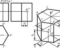
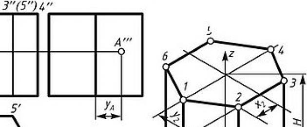
Hexagonal prism in isometry. The construction of a hexagonal prism according to this drawing in a system of orthogonal projections (on the left in Fig. 6.7) is shown in Fig. 6.7. On the isometric axis I put off height H, draw lines parallel to the axes hiu. Mark on a line parallel to the axis X, position of points / and 4.

To build a point 2 determine the coordinates of this point in the drawing - x 2 and at 2 and, setting aside these coordinates on the axonometric image, build a point 2. Points are built in the same way. 3, 5 and 6.

The constructed points of the upper base are connected to each other, an edge is drawn from the point / to the intersection with the x-axis, then -

dotted edges 2 , 3, 6. The ribs of the lower base are drawn parallel to the ribs of the upper one. Building a point L, located on the side face, along the coordinates x A(or at A) and 1 A evident from

Circle isometry. Circles in isometry are depicted as ellipses (Fig. 6.8) indicating the values ​​of the axes of the ellipses for the reduced distortion coefficients equal to one.

The major axis of the ellipses is at 90° for ellipses lying IN THE PLANE xC>1 to OSI y, IN THE PLANE y01 TO X-AXIS, in plane hoy To OSI?

When constructing an isometric image by hand (like a drawing), an ellipse is performed at eight points. For example, trays 1, 2, 3, 4, 5, 6, 7 and 8 (see figure 6.8). points 1, 2, 3 and 4 are found on the corresponding axonometric axes, and the points 5, 6, 7 and 8 are built according to the values ​​of the corresponding major and minor axes of the ellipse. When drawing ellipses in isometric projection, you can replace them with ovals and build them as follows 1 . The construction is shown in fig. 6.8 on the example of an ellipse lying in a plane xOz. From the point / as from the center, make a notch with a radius R=D on the continuation of the minor axis of the ellipse at the point O, (they also build a point symmetrical to it in the same way, which is not shown in the drawing). From point O, how to draw an arc from the center CGC radius D, which is one of the arcs that make up the contour of the ellipse. From point O, as from the center, an arc of radius is drawn O^G to the intersection with the major axis of the ellipse at points OU Passing through the points O p 0 3 straight line, found at the intersection with the arc CGC point TO, which defines 0 3 K- the value of the radius of the closing arc of the oval. points To are also the conjugation points of the arcs that make up the oval.

Cylinder isometric. The isometric image of a cylinder is determined by the isometric images of the circles of its base. Construction in isometry of a cylinder with a height H according to the orthogonal drawing (Fig. 6.9, left) and the point C on its side surface is shown in fig. 6.9, right.

Suggested by Yu.B. Ivanov.

An example of construction in an isometric projection of a round flange with four cylindrical holes and one triangular one is shown in fig. 6.10. When constructing the axes of cylindrical holes, as well as the edges of a triangular hole, their coordinates were used, for example, the coordinates x 0 and y 0 .

Instruction

Construct with a ruler and protractor or a compass and ruler for a rectangular (orogonal) isometric projection. In this type of axonometric projection, all three axes - OX, OY, OZ - are angles of 120 ° to each other, while the OZ axis has a vertical orientation.

For simplicity, draw an isometric projection without distortion along the axes, since it is customary to equate the isometric distortion factor to one. By the way, “isometric” itself means “equal size”. In fact, when displaying a three-dimensional object on a plane, the ratio of the length of any projected segment parallel to the coordinate axis to the actual length of this segment is equal to 0.82 for all three axes. Therefore, the linear dimensions of the object in isometry (with the accepted distortion coefficient) increase by 1.22 times. In this case, the image remains correct.

Start projecting the object onto the axonometric plane from its top face. Measure along the OZ axis from the center of intersection of the coordinate axes the height of the part. Draw thin lines for the X and Y axes through this point. From the same point, set aside half the length of the part along one axis (for example, along the Y axis). Draw a segment of the required size (part width) through the found point parallel to the other axis (OX).

Now, along the other axis (OX), set aside half the width. Through this point, draw a segment of the desired size (part length) parallel to the first axis (OY). The two drawn lines must intersect. Complete the rest of the top face.

If this face has a round hole, draw it. In isometry, a circle is shown as an ellipse because we are looking at it from an angle. Calculate the dimensions of the axes of this ellipse based on the diameter of the circle. They are equal: a = 1.22D and b = 0.71D. If the circle is located on a horizontal plane, the a-axis of the ellipse is always horizontal, the b-axis is always vertical. In this case, the distance between the points of the ellipse on the X or Y axis is always equal to the diameter of the circle D.

Draw from the three corners of the top face vertical edges equal to the height of the part. Connect the edges through their bottom points.

If the shape has a rectangular hole, draw it. Set aside a vertical (parallel to the Z axis) segment of the desired length from the center of the edge of the upper face. Through the resulting point, draw a segment of the required size parallel to the upper face, and hence the X axis. From the extreme points of this segment, draw vertical edges of the desired size. Connect their bottom points. From the lower right point of the drawn rhombus, draw the inner edge of the hole, which should be parallel to the Y axis.

6.1. General provisions

Complex (technical) drawings are built according to the method of rectangular projection on the projection plane, while the number of images of the object in these drawings should be the smallest, but fully revealing its shape and dimensions. Such drawings are reversible, measurable, but not visual enough, since the spatial image of an object in the mind very often has to be reproduced from several of its images. Therefore, there was a need for drawings that would be visual, but at the same time reversible and give a general idea of ​​the relative size and shape of the object.

An axonometric projection is a visual image of an object obtained by parallel projecting it onto one axonometric projection plane P together with axes of the spatial coordinate system Oxyz to which it belongs (an object is assigned to a coordinate system if its projection onto one of the coordinate planes is known.). Projection

that on the plane P called axonometric (axonometry);

projections of coordinate axes - corresponding axonometric axes(they are simply referred to as x, y, z instead of x, y, z); the ratio of the length of the axonometric projection of a segment parallel to the coordinate axis to the natural length of the segment - distortion indicator along the corresponding axonometric axis. If the direction of projection is perpendicular to the plane P, then the axonometry is called rectangular, and if not, then oblique.

To build visual technical images, GOST 2.317-69 * recommends standard axonometries that have good visibility.

6.2. Rectangular Isometric View(isometry)

This type of axonometry is obtained with the same inclination of all coordinate planes associated with the object to the axonometric projection plane. Therefore, in isometry, the distortion coefficients along the x, y and z axes are the same (they are equal to 0.82), and the axonometric axes form angles of 120° between themselves (Fig. 6.1). They can be built using a compass or squares with

		angles 30O and 60O, placing
		z-axis is vertical. On fig.
		6.1 the x and y axes are drawn with
		slope 4:7 to the horizontal
		line of the drawing.
		To simplify isomet-
		Riya is built using the
		given indicators of distortion
		along the axes equal to 1. In this
		case image of the subject
		in isometry	performed in
		scaled up 1.22:1.
		Rectangular isomet-
		ria is most convenient for
		items	curvilinear
		shape, length, width and
	the height of which differ from each other not very significantly.
	6.3. Rectangular dimetric projection
		(dimetria)

Dimetry is obtained with the same inclination to the axonometric plane of the coordinate planes xOy and yOz, therefore, the distortion indicators along the x and z axes are the same and equal to 0.94, and along the y axis - 0.47. Using in practice the given distortion indicators (1 each for the x and z axes and 0.5 for the y axis), the dimetry is performed on an enlarged scale

ratio 1.06:1.

When constructing axonometric axes (Fig. 6.2), the axis

z is carried out vertically, and for

plotting the x and y axes
it is not the angles of their inclination to the horizontal
umbrella line
(respectively 7 10 and
and their biases towards this
(respectively 1:8 and 7:8).
Rectangular dimetria
appropriate to apply
prismatic and

pyramidal shapes, as well as for elongated objects, in which the length significantly exceeds the width and height, directing the length parallel to the x or z axis. In this case, the length is not subjected to strong distortion and the idea of ​​the shape of the object and the ratio of its main dimensions is not lost.

6.4. Drawing circles in axonometry

A circle lying in the coordinate plane or a plane parallel to it is projected in a rectangular axonometry into an ellipse, the major axis of which is perpendicular to the “free” axonometric axis, and the minor one is parallel to it. A free axonometric axis is a projection of the coordinate axis perpendicular to the plane of the circle (for example, for a circle whose plane is parallel to the yOz plane, the x-axis is the “free” axis).

The construction of the given indicators of distortion of ellipses into which circles are projected, the planes of which are parallel to the coordinate ones, is shown for standard isometry and dimetry in fig. 6.1 and 6.2 respectively.

The major axes of these ellipses in isometry are 1.22d, and the minor axes are 0.71d (d is the diameter of the circle). Ellipses in isometry (Fig. 6.1) are built along major and minor axes (4 points) and points on diameters parallel to the coordinate axes (4 more points).

In dimetry, the major axes of the ellipses are equal to 1.06d, and the minor axes are equal to 0.35d for circles lying in the xOy and yOz planes and parallel to them, and 0.94d for circles located in the xOz plane and planes parallel to it. To construct ellipses in dimetry, 8 points are used, similar to the points along which an ellipse is drawn in isometry (Fig. 6.2). To more accurately build ellipses into which circles are projected parallel to the xOy and yOz planes, additional points are used, obtained due to the symmetry of the points of the ellipses relative to the major and minor axes.

On fig. 6.1 and 6.2, near the axes of the ellipses and their diameters, the reduced distortion indicators in these directions are indicated.

Axonometric projections of circles (arcs) of large radius, circles that do not lie in planes parallel to the coordinate ones, and curved lines are built according to the axonometric projections of their points.

6.5. Examples of axonometric projections of various objects

The axonometry of an object is usually built according to its technical drawing, on which the projections of the axes of the spatial coordinate system Oxyz, to which the object is assigned, can be indicated.

The construction of axonometry begins with the axonometric axes.

Axonometric projections of figures are built on axonometric projections of their characteristic points. Axonometric projections of points are built according to the coordinates of these points, taking into account the distortion indicators along the axonometric axes.

Axonometric projections of segments are built on axonometric projections of their two points. Axonometric projections of parallel lines are parallel. In this case, the axonometric projections of lines parallel to the coordinate axes are parallel to the corresponding axonometric axes and have the same distortion indicators.

On fig. 6.3a, 6.4a and 6.5a are technical drawings of the parallelepiped, hemisphere and cone of revolution, respectively, in fig. 6.3b and 6.4b show isometries of the first two figures, and in fig. 6.5b - dimetry of the third.

A 1 E 1

a) z 2

a) z 2

a) z

x

The outline of a sphere in a rectangular projection is always a circle with a radius equal to the radius of the sphere R. When using the given distortion indicators, the radius of the outline of the sphere in isometry is increased to 1.22R, and in dimetry - up to 1.06R.

When constructing the axonometry of an object, they try, if possible, to align the coordinate plane xOy with the plane of the base of the object, and the coordinate axes with its edges or axes of symmetry.

On fig. 6.6a and 6.7a are complex drawings of objects, and in fig. 6.6c and 6.7b, respectively, are isometric projections of these objects with a cutout of one quarter.

Cut-outs in axonometric images are necessary in the same way as cuts in technical drawings, in order to reveal the hidden internal forms of the object.

Sections in axonometry can be built in two ways. The first way is to build a complete image

object in thin lines, followed by drawing the contours of the sections formed by each cutting plane of the cutout, and removing the image of the cut-off part of the object (Fig. 6.6b).

According to the second method, the contours of the sections of the object are first built by cutting planes (shown in Fig. 6.6b by the main lines), and then the image of the rest of the object is performed.

In axonometry, as a rule, do not use full cuts, in which at least one of the three main dimensions of the object disappears(length Width Height). Otherwise, axonometry would be deprived of its main advantage - clarity.

To determine the direction of hatching in sections on the axonometric axes, an arbitrary segment b is laid, and in dimetry on the y axis, half of this segment. The straight lines connecting the ends of the segments set the hatching direction for the corresponding planes (Fig. 6.1 and 6.2).

If the cutting plane passes through stiffeners, solid protrusions or thin walls, then the sections of these part elements are always shaded. In axonometry, holes located on round flanges or disks are not rotated into the cut plane (Fig. 6.6).

AT axonometry, it is allowed not to show small structural elements of the object (chamfers, fillets, etc.). The lines of a smooth transition from one surface to another are shown by conditionally thin lines (Fig. 6.7b).

Lecture 6

1. General information about axonometric projections.

2. Classification of axonometric projections.

3. Examples of constructing axonometric images.

1 Introduction to axonometric projections

When drawing up technical drawings, sometimes it becomes necessary, along with images of objects in the system of orthogonal projections, to have more visual images. For such images, the method axonometric projection(axonometry is a Greek word, in literal translation it means measurement along the axes; axon - axis, metereo - I measure).

The essence of the method of axonometric projection: the object, together with the axes of rectangular coordinates to which it is referred in space, is projected onto a certain plane so that none of its coordinate axes is projected onto it into a point, which means that the object itself is projected onto this projection plane in three dimensions.

Damn it. 88 onto a certain plane of projections P, a coordinate system x, y, z located in space is projected. Projections x p , y p ,

z p coordinate axes to the plane P are called axonometric axes.

Figure 88

Equal segments e are plotted on the coordinate axes in space. As can be seen from the drawing, their projections e x, e y, e z onto the plane P in general

case are not equal to the segment e and are not equal to each other. This means that the dimensions of the object in axonometric projections along all three axes are distorted. The change in linear dimensions along the axes is characterized by indicators (coefficients) of distortion along the axes.

Distortion indicator is the ratio of the length of a segment on an axonometric axis to the length of the same segment on the corresponding axis of a rectangular coordinate system in space.

The distortion index along the x axis will be denoted by the letter k, along the y axis

- the letter m, along the z axis - the letter n, then: k = e x / e; m = e y /e; n = e z /e.

The magnitude of the distortion indicators and the ratio between them depend on the location of the projection plane and on the projection direction.

In the practice of constructing axonometric projections, they usually use not the distortion coefficients themselves, but some values ​​proportional to the values ​​of the distortion coefficients: K:M:N = k:m:n. These quantities are called given distortion coefficients.

2 Classification of axonometric projections

The whole set of axonometric projections is divided into two groups:

1 Rectangular projections - obtained with a projection direction perpendicular to the axonometric plane.

2 Oblique projections - obtained with the projection direction selected at an acute angle to the axonometric plane.

In addition, each of these groups is also divided according to the ratio of axonometric scales or indicators (coefficients) of distortion. On this basis, axonometric projections can be divided into the following types:

a) Isometric - distortion indicators for all three axes are the same (isos - the same).

b) Dimetric - distortion indicators along two axes are equal to each other, and the third one is not equal (di - double).

c) Trimetric - distortion indicators on all three axes are not equal

us among ourselves. This is axonometry (it has no great practical application).

2.1 Rectangular axonometric projections

Rectangular Isometric View

AT rectangular isometry, all coefficients are equal between

k = m = n , k2 + m2 + n2 =2 ,

then this equality can be written as 3k 2 =2 , whence k = .

Thus, in isometry, the distortion index is ~ 0.82. This means that in a rectangular

isometry, all dimensions of the depicted object are reduced by 0.82 times. For

simplification	constructions		use
given	odds		distortion
k=m=n=1,		corresponds
increase	sizes	images by
compared with the actual ones in 1.22
times (1:0.82		Axle arrangement
isometric projection is shown in fig.
			Figure 89

Rectangular dimetric projection

In rectangular dimetry, the distortion indicators along the two axes are the same, i.e. k \u003d n. Third

we choose the distortion index half as much as the other two, i.e. m = 1/2k. Then the equality k 2 +m 2 +n 2 = 2 will take the following form: 2k 2 +1/4k 2 =2; whence k= 0.94;

	m = 0.47.
	In order to simplify the construction
	use	given
	distortion coefficients: k=n=1 ;
	m=0.5 . The increase in this case
	is 6% (expressed as a number		Figure 90
	1,06=1:0,94).	Axle arrangement
	dimetric	projection shown in

Figure 91

Figure 92

are equal: k = n=1.

2.2 Oblique projections

Frontal isometric view

On fig. 91 the position of axonometric axes for frontal isometry is given.

According to GOST 2.317-69, it is allowed to use frontal isometric projections with an angle of inclination of the y-axis of 30° and 60°. The distortion coefficients are exact and equal to:

k = m = n=1.

Horizontal isometric view

On fig. 92 the position of axonometric axes for frontal isometry is given. According to GOST 2.317-69, it is allowed to use horizontal isometric projections with a tilt angle of the y axis of 45° and 60° while maintaining the angle between the x and y axes of 90°. The distortion coefficients are exact and equal: k=m= n= 1 .

Frontal dimetric projection

The position of the axes is the same as for the frontal isometry (Fig. 91). It is also allowed to use frontal dimetry with 30° and 60° y-axis inclination.

The distortion coefficients are accurate and m=0.5

All three types of standard oblique projections were obtained with one of the coordinate planes (horizontal or frontal) parallel to the axonometric plane. Therefore, all figures located in these planes or parallel to them are projected onto the plane of the drawing without distortion.

3 Examples of constructing axonometric images

Both in rectangular (orthogonal) and axonometric projections, one projection of a point does not determine its position in space. In addition to the axonometric projection of a point, it is necessary to have another projection, called the secondary one. Secondary Point Projection- this is an axonometry of one of its rectangular projections (usually horizontal).

Techniques for constructing axonometric images do not depend on the type of axonometric projections. For all projections, the methods of construction are the same. An axonometric image is usually built on the basis of rectangular projections of an object.

3.1 Axonometry of a point

The construction of the axonometry of a point according to its given orthogonal projections (Fig. 93, a) begins with the definition of its secondary projection (Fig. 93, b). To do this, on the axonometric axis x from the origin, we set aside the value of the X coordinates of the point A - X A; along the y axis - the segment Y A (for the dimetry Y A ×0.5, since the distortion index along this axis is m=0.5).

At the intersection of communication lines drawn parallel to the axes from the ends of the measured segments, a point A 1 is obtained - a secondary projection of the point A.

The axonometry of point A will be at a distance Z A from the secondary projection of point A.

Figure 93

3.2 Axonometry of a straight line segment (Fig. 94)

We find secondary projections of points A, B. To do this, we set aside along the x and y axes the corresponding coordinates of points A and B. Then mark on straight lines drawn from secondary projections parallel to the z axis, the heights of points A and B (Z A and Z B). We connect the points obtained - we get the axonometry of the segment.

Figure 94

3.3 Axonometry of a plane figure

On fig. 95 shows the construction of an isometric projection of the triangle ABC. We find secondary projections of points A, B, C. To do this, we set aside along the x and y axes the corresponding coordinates of points A, B and C. Then we mark on the straight lines drawn from the secondary projections parallel to the z axis, the heights of points A, B and C. We connect the obtained points with lines - we get the axonometry of the segment.

Figure 95

If a flat figure lies in the plane of projections, then the axonometry of such a figure coincides with its projection.

3.4 Axonometry of circles located in projection planes

Circles in axonometry are depicted as ellipses. To simplify the constructions, the construction of ellipses is replaced by the construction of ovals outlined by arcs of circles.

Rectangular circle isometry

	On fig. 96 in		rectangular
	isometric depiction of a cube, in the face
	whom			circles.
			rectangular
	isometries will be rhombuses, and
	circles are ellipses. Length
	the major axis of the ellipse is 1.22d,
	where d is the diameter of the circle. Malaya
	the axis is 0.7 d .
				shown
	construction of an oval lying in
	plane parallel to π 1 . From
	the points of intersection of the axes O spend
	auxiliary			circle	Figure 96
	diameter d, equal to the actual

the nominal value of the diameter of the depicted circle, and find the points n of intersection of this circle with the axonometric axes x and y.

From the points O 1, O 2 of the intersection of the auxiliary circle with the z axis, as

from centers with a radius R \u003d O 1 n \u003d O 2 n, two arcs nDn and pSp of the circle belonging to the oval are drawn.

	From the center O with radius OS ,
	equal to half the minor axis of the oval,
	mark on the major axis of the oval
	points O 3 and O 4. From these points
	radius r = O3 1 = O3 2 = O4 3
	About 4 4 spend two arcs. Points 1, 2, 3
	and 4 conjugations of arcs of radii R and r
	find by connecting the points O 1 and O 2 with
	points O 3 and O 4 and continuing		Figure 97
	straight lines to the intersection with arcs
	pSp and nDn.
	Ovals are built in the same way,		located in
	planes parallel to the planes π 2,		and π 3, (Figure 98).

The construction of ovals lying in planes parallel to the planes π 2 and π 3 begins with the horizontal AB and vertical CD axes of the oval:

AB axis x for an oval lying in a plane parallel to the planes π 3 ;

AB axis y for an oval lying in a plane parallel to

planes π 2 ; Further construction of ovals is similar to the construction of an oval,

lying in a plane parallel to π1.

Figure 98

Rectangular dimetry of the circle (Fig. 99)

On fig. 99 in a rectangular isometry, a cube with an edge α is shown, in the faces of which circles are inscribed. Two faces of the cube will be depicted as equal parallelograms with sides equal to 0.94d and 0.47d, the third face - in the form of a rhombus with sides equal to 0.94d. Two circles inscribed in the faces of a cube are projected as identical ellipses, the third ellipse is close to a circle in shape.

Direction of large
ellipses (as in isometry)
perpendicular
relevant axonometric
axes, minor axes are parallel
axonometric axes.
three ellipses is
circle diameter,
minor axes		identical
ellipses are d/3		small size
axis of an ellipse close in shape to
circles,				0.9d.
Practically		given
distortion indicators			(1 and	0,5)	Figure 99
major axes of all three ellipses

are 1.06 d, the minor axes of the two ellipses are 0.35 d, the minor axis of the third ellipse is 0.94 d.

Building ellipses			in dimetria is sometimes replaced by more
simple construction of ovals (Fig. 100)
Figure 100		examples of constructing dimetric
projections,		ellipses are replaced			built
simplified	way.		Consider		building

dimetric projection of a circle located parallel to the plane π 2 (Figure 100, a).

Through point O we draw axes parallel to the x and z axes. From the center O with a radius equal to the radius of the given circle, we draw an auxiliary circle that intersects with the axes at points 1, 2, 3, 4. From points 1 and 3 (in the direction of the arrows) we draw horizontal lines until they intersect with the axes AB and CD of the oval and get points O 1, O 2, O 3, O 4. Taking the points О 1, О 4 as centers, we draw arcs 1 2 and 3 4 with radius R. Taking the points О 2, О 3 as centers, we draw the arcs closing the oval with a radius R 1.

Let us analyze the simplified construction of the dimetric projection of a circle lying in the plane π 1 (Figure 100, c).

Through the intended point O we draw straight lines parallel to the x and y axes, as well as the major axis of the oval AB perpendicular to the minor axis CD. From the center O with a radius equal to the radius of the given circle, we draw an auxiliary circle and get points n and n 1.

On a straight line parallel to the z axis, to the right and left of the center O

set aside segments equal to the diameter of the auxiliary circle, and get the points O 1 and O 2. Taking these points as centers, we draw the arcs of ovals with a radius R \u003d O 1 n 1. Connecting the points O 2 with straight lines to the ends of the arc n 1 n 2, on the line of the major axis AB of the oval we get points O 4 and O 3. Taking them as centers, we draw an arc closing the oval with a radius R 1.

Figure 100

3.5 Axonometry of a geometric body

Axonometry of a hexagonal prism (Fig. 101)

The base of a right prism is a regular hexagon

Construction of an axonometric image of a part, the drawing of which is shown in Fig.a.

All axonometric projections must be performed in accordance with GOST 2.317-68.

Axonometric projections are obtained by projecting an object and its associated coordinate system onto one projection plane. Axonometries are divided into rectangular and oblique.

For rectangular axonometric projections, the projection is perpendicular to the projection plane, and the object is positioned so that all three planes of the object are visible. This is possible, for example, when the axes are located, as on a rectangular isometric projection, for which all projection axes are located at an angle of 120 degrees (see Fig. 1). The word "isometric" projection means that the coefficient of distortion in all three axes is the same. According to the standard, the distortion coefficient along the axes can be taken equal to 1. The distortion coefficient is the ratio of the size of the projection segment to the true size of the segment on the part, measured along the axis.

Let's build an axonometry of the part. First, let's set the axes, as for a rectangular isometric projection. Let's start from the foundation. Let us set aside the value of the length of the part 45 along the x-axis, and the value of the width of the part 30 along the y-axis. On axonometric images, when applying dimensions, extension lines are drawn parallel to the axonometric axes, dimension lines - parallel to the measured segment.

Next, we draw the diagonals of the upper base and find the point through which the axis of rotation of the cylinder and the hole will pass. We erase the invisible lines of the lower base so that they do not interfere with our further construction (Fig. 3)

.

The disadvantage of a rectangular isometric projection is that the circles in all planes will be projected into ellipses on the axonometric image. Therefore, first we will learn how to build approximately ellipses.

If a circle is inscribed in a square, then 8 characteristic points can be marked in it: 4 points of contact between the circle and the middle of the side of the square and 4 points of intersection of the diagonals of the square with the circle (Fig. 4, a). Fig. 4c and Fig. 4b show the exact way of constructing the points of intersection of the diagonal of a square with a circle. Figure 4e shows an approximate method. When constructing axonometric projections, half of the diagonal of the quadrilateral into which the square is projected will be divided in the same ratio.

We transfer these properties to our axonometry (Fig. 5). We build a projection of a quadrilateral into which a square is projected. Next, we build an ellipse Fig.6.

Next, we rise to a height of 16mm and transfer the ellipse there (Fig. 7). We remove extra lines. We turn to the construction of holes. To do this, we build an ellipse at the top, into which a hole with a diameter of 14 is projected (Fig. 8). Further, in order to show a hole with a diameter of 6 mm, it is necessary to mentally cut out a quarter of the part. To do this, we will build the middle of each side, as in Fig. 9. Next, we build an ellipse corresponding to a circle with a diameter of 6 on the lower base, and then at a distance of 14 mm from the upper part of the part we draw already two ellipses (one corresponding to a circle with a diameter of 6, and the other corresponding to a circle with a diameter of 14) Fig.10. Next, we cut a quarter of the part and remove invisible lines (Fig. 11).

Let's proceed to the construction of the stiffener. To do this, on the upper plane of the base, we measure 3 mm from the edge of the part and draw a segment half the thickness of the rib (1.5 mm) long (Fig. 12), we also mark the rib on the far side of the part. An angle of 40 degrees does not suit us when constructing axonometry, so we calculate the second leg (it will be equal to 10.35mm) and build the second point of the angle along the plane of symmetry using it. To build the border of the rib, we build a straight line at a distance of 1.5mm from the axis on the upper plane of the part, then we draw the lines parallel to the x-axis until they intersect with the outer ellipse and lower the vertical straight line. Draw a straight line through the lower point of the rib boundary parallel to the rib along the cut plane (Fig. 13) until it intersects with the vertical line. Next, we connect the intersection point with a point in the cut plane. To construct the far edge, we draw a straight line parallel to the X axis at a distance of 1.5 mm to the intersection with the outer ellipse. Next, we find the distance at which the upper point of the rib boundary is (5.24mm) and set aside the same distance on a vertical straight line from the far side of the part (see Fig. 14) and connect it to the far lower point of the rib.

We remove the extra lines and hatch the section planes. The hatching lines of sections in axonometric projections are applied parallel to one of the diagonals of the projections of squares lying in the corresponding coordinate planes, the sides of which are parallel to the axonometric axes (Fig. 15).

For a rectangular isometric projection, the hatch lines will be parallel to the hatch lines shown in the diagram in the upper right corner (Fig. 16). It remains to depict the side holes. To do this, we mark the centers of the axes of rotation of the holes, and build ellipses, as indicated above. Similarly, we build rounding radii (Fig. 17). The final axonometry is shown in Fig.18.

For oblique projections, projection is carried out at an angle to the projection plane, other than 90 and 0 degrees. An example of an oblique projection is the oblique frontal dimetric projection. It is good because on the plane given by the X and Z axes, circles parallel to this plane will be projected to the true value (the angle between the X and Z axes is 90 degrees, the Y axis is tilted at an angle of 45 degrees to the horizon). "Dimetric" projection means that the coefficients of distortion along the two axes X and Z are the same, along the Y axis the coefficient of distortion is two times less.

When choosing an axonometric projection, it is necessary to strive for the largest number of elements to be projected without distortion. Therefore, when choosing the position of a part in an oblique frontal dimetric projection, it must be positioned so that the axes of the cylinder and holes are perpendicular to the frontal projection plane.

The layout of the axes and the axonometric image of the part "Rack" in an oblique frontal dimetric projection is shown in Fig.18.